
How many hawker stalls are a walking distance from me?
With the current situation in the world being what it is and any chance of entering and leaving Singapore seems off the table for foreseeable future, since our lockdown was lifted last month I’ve been playing catchup on exploring Singapore in greater detail. While exploring all the famous hawker centres was one of the first things I dove into when I first moved to Singapore last year, my busy work and travel schedule put it on the backburner for a while. Now more time to explore local neighbourhoods has meant more time to eat. So I wanted to see how many possible hawker centres were within my vicinity and to test out some new R packages I had been meaning to try.
This interactive map shows how many hawker centres and hawker centre stalls there are within a 30 minute walk of any point in Singapore. The map is rendered in deck.gl using the mapdeck R package. Data for walking isochrones comes from mapbox and generated for each hawker centre using the brand new mapboxapi package. Spatial indexing is done using the geohashTools package. All code including this page is written in R and is documented step-by-step at the bottom of the page (scroll on, if interested.)
A few caveats: people seldom walk 30 minutes to get anywhere in Singapore – it’s too hot. Also, the data here is based on the data for government run hawker centres using data from data.gov.sg. While extensive - there are 114 hawker centres comprising around 6400 individual food stalls, this does not include the countless stalls and kopitiams (“coffee shops”) scattered around the island under residential housing blocks and commercial towers. The actual count of hawkers and hawker-like stalls in the country must be close to 10,000 – if not more.
The map below is interactive, zoomable, and provides detail for each location on mouseover. This might take a few seconds to load, especially on older devices. A full-screen version is available at https://www.dshkol.com/hawker-accessibility-map.html which will take about 15-20s to fully render, depending on device.
Based on this, from my building I have access to around 1028 hawker stalls from 15 different hawker centres. Not bad! Somewhere just to the west of Tiong Bahru Market is the place in Singapore with the greatest number of accessible food stalls within a 30m walk - 1352 stalls from 19 different markets.
Hawker centres and their role in Singaporean culture
Hawker food is an integral part of day to life for Singaporeans and is generally what people think of when they think of Singapore as a foodie destination. The Singaporean government began to move street food vendors and hawkers into indoor centres from the 1950s onward. As a result, there is relatively very little true street food in Singapore, especially compared to other cities in SE Asia. But that transition from outdoor street food into complexes created its own cultural touchstone - the hawker centre.
Hawker centres are complexes, mostly indoor although some are partially outdoors, that contain a large number of food and market stalls. Most food stalls are small in size and specialize in a particular dish or cuisine, and everyone has their own opinions about which ones are best. The largest hawker centres will have several hundred food stalls, while small ones might only have a dozen. These places function as more than a place to eat, however. Hawkers are, in essence, a community place, a third-space, and a preservation of food culture. Singapore is currently trying to get hawker culture recognized as an officially recognized UNESCO intangible culture.
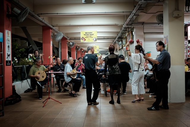
Evenings at Golden Mile Food Centre
This is an easy way to start a fight but my own top favourites are:
- Old Airport Road Food Centre
- Golden Mile Food Centre
- Maxwell Food Centre
- Chinatown Complex
- Zion Riverside
How this is made: step-by-step code breakdown
Getting and processing the data
All data for this project comes from https://data.gov.sg/. Hawker centre geography and details are from the most recently updated public data. Singapore geography is from the electoral boundary files. I usually find this dataset more useful than the national map one because it excludes all the minor outlying islands that can distort maps of Singapore. Both datasets are rehosted on my own github gist to make it easier to reproduce repeatedly.
# Get hawker centres spatial data
library(sf)

# I've rehosted geojson the hawker dataset from data.gov.sg as a github gist
hawkers <- read_sf("https://gist.github.com/dshkol/68751598a52ca28a52b24ff61aa5126d")
The description field contains useful data about each hawker centre that we need in order to get the names and the number of stalls; however, it’s all a bunch of HTML so we use some simple regex to extract.
library(stringr)
library(dplyr)
# Get name and number of stalls using our friend regular expressions
hawkers <- hawkers %>%
  mutate(
    id = c(1:length(hawkers$geometry)),
    name = str_extract(Description,"(?<=<th>NAME</th> <td>)(.*?)(?=</td>)"),
    status = str_extract(Description,"(?<=<th>STATUS</th> <td>)(.*?)(?=</td>)"),
    no_food_stalls = as.numeric(
      str_extract(
        Description,
        "(?<=<th>NO_OF_FOOD_STALLS</th> <td>)(.*?)(?=</td>)")),
    no_market_stalls = as.numeric(
      str_extract(
        Description,
        "(?<=<th>NO_OF_MARKET_STALLS</th> <td>)(.*?)(?=</td>)")))

head(hawkers)
## Simple feature collection with 6 features and 7 fields
## geometry type: POINT
## dimension: XYZ
## bbox: xmin: 103.8142 ymin: 1.320648 xmax: 103.887 ymax: 1.36824
## z_range: zmin: 0 zmax: 0
## geographic CRS: WGS 84
## # A tibble: 6 x 8
## Name Description geometry id name status no_food_stalls
## <chr> <chr> <POINT [°]> <int> <chr> <chr> <dbl>
## 1 kml_1 "<center><… Z (103.8142 1.324134 0) 1 Adam… Exist… 32
## 2 kml_2 "<center><… Z (103.887 1.320648 0) 2 Alju… Exist… 79
## 3 kml_3 "<center><… Z (103.8392 1.366788 0) 3 Ang … Exist… 10
## 4 kml_4 "<center><… Z (103.8483 1.364105 0) 4 Ang … Exist… 32
## 5 kml_5 "<center><… Z (103.8554 1.362769 0) 5 Ang … Exist… 40
## 6 kml_6 "<center><… Z (103.8564 1.36824 0) 6 Ang … Exist… 39
## # … with 1 more variable: no_market_stalls <dbl>The data also includes under construction and proposed hawker centres. Let’s exclude those for now.
# Exclude U/C and proposed
hawkers <- hawkers %>%
  filter(!status %in% c("Proposed",'Under Construction'))
What does this look like? Let’s grab some Singapore geo data (using the electoral boundary dataset here) to use as a base map here.
library(ggplot2)

sg_map <- read_sf("https://gist.github.com/dshkol/d3e1dcaad80f7010d73ddc397052c075")
sg_map <- st_zm(sg_map) # remove Z dimension

ggplot() +
  geom_sf(data = sg_map, fill = "white") +
  geom_sf(data = hawkers, aes(size = no_food_stalls), alpha = 0.5)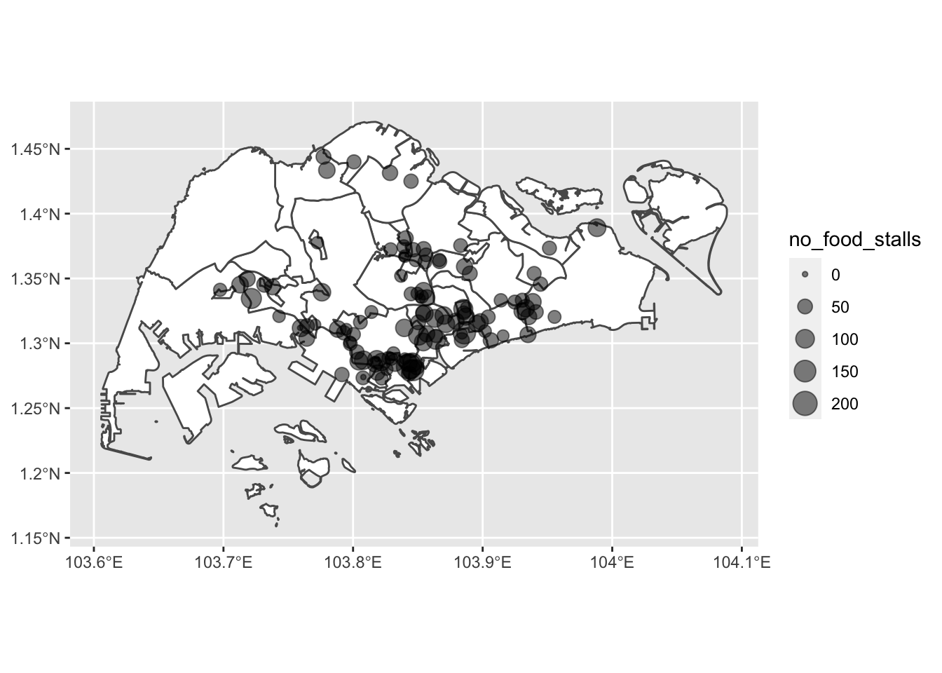
Generating walking isochrones with mapboxapi
Next we want to generate the walksheds for each hawker centre. Time-measured walksheds are known as isochrones, and these can be generated by routing services. Here, we turn to the Mapbox navigation API. The mapboxapi package by Kyle Walker provides R bindings for various Mapbox API services, including isochrones. Mapbox API usage requires an API key, but their free level key is quite generous in usage. I generally store my API keys in my .Renviron file and load them via Sys.getenv(...).
The package has a function mb_isochrone which takes as arguments a pair of coordinates, a time shed, and a travel profile (i.e. walking, driving, cycling).
library(mapboxapi)

# get lat lon of hawkers using st_coordinates
xy <- st_coordinates(hawkers[1,])

iso30 <- mb_isochrone(
    location = c(xy[1], xy[2]),
    profile = "walking",
    time = 30,
    access_token = Sys.getenv("MAPBOX_API_KEY")
  )

iso15 <- mb_isochrone(
    location = c(xy[1], xy[2]),
    profile = "walking",
    time = 15,
    access_token = Sys.getenv("MAPBOX_API_KEY")
  )

# Visualizing isochrones for 15 and 30 minute walksheds around Adam Road Food Centre
ggplot() +
  geom_sf(data = sg_map, fill = "white") +
  geom_sf(data = hawkers[1,]) +
  geom_sf(data = iso30, fill = "green", alpha = 0.5) +
  geom_sf(data = iso15, fill = "orange", alpha = 0.5)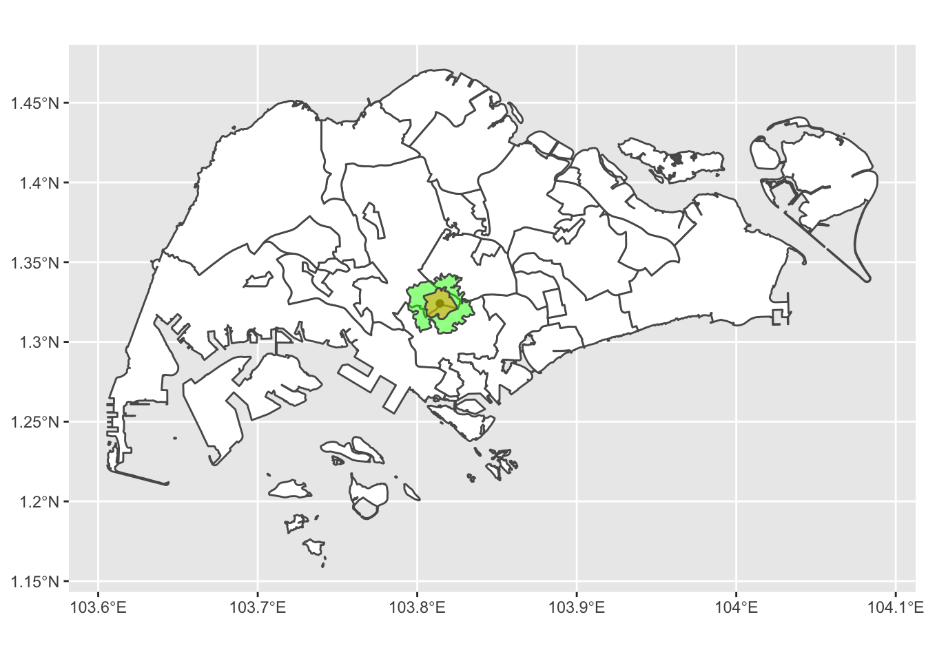
Because I want to iterate this across a bunch of hawker centres at once that I have as a POINT collection, I write my own function here that makes it easy to do this at scale and store the data I need in a tidy object.
# Calculate isochrones for each hawker centre
get_isochorones <- function(shed = 30, i) {
  # Get coords
  sel_hawker  <- hawkers[i, ]

  coords <- st_coordinates(hawkers[i, ])

  iso <- mb_isochrone(
    location = c(coords[1], coords[2]),
    profile = "walking",
    time = shed,
    access_token = Sys.getenv("MAPBOX_API_KEY")
  )
  iso %>%
    mutate(
      id = sel_hawker$id,
      name = sel_hawker$name,
      no_food_stalls = sel_hawker$no_food_stalls,
      no_market_stalls = sel_hawker$no_market_stalls
    )
}
With this function ready, I use purrr:map2_df to feed a list of hawker centres from my POINT collection along with a time parameter and my custom function get_isochrones. The results of this end up in a nice and tidy simple feature collection of polygons representing the isochrone for each hawker centre.
library(purrr)
# Iterate for
# hawker15 <- map2_df(15, c(1:length(hawkers$id)), get_isochorones) # if we want to do 15 min sheds instead
hawker30 <- map2_df(30, c(1:length(hawkers$id)), get_isochorones)

ggplot() +
  geom_sf(data = sg_map, fill = "white") +
  geom_sf(data = hawkers) +
  geom_sf(data = hawker30, fill = "orange", colour = NA, alpha = 0.10)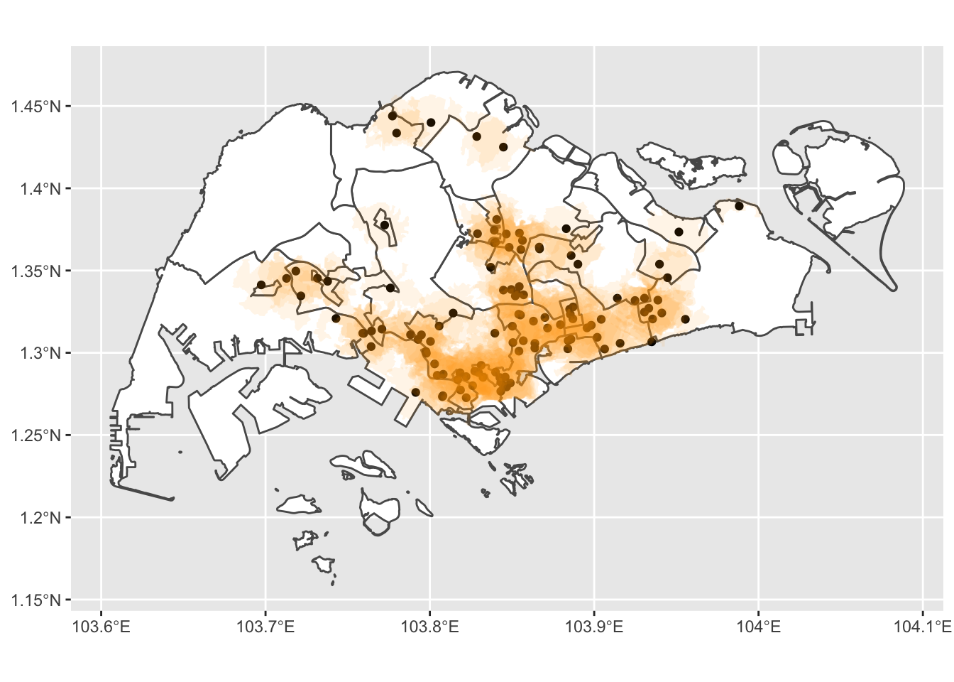
Creating a spatial reference with geohashTools
We can subdivide the geography we are working with to have a spatial index as a frame of reference. There are a number of different spatial indexing libraries out in the wild and it would make for a good post on its own. I tend to use geohashes because it makes for nice grids that don’t have much distortion at Singapore latitudes. There is an R package geohashTools written by my colleague Michael Chirico and that I’ve made some small contributions to. Geohashes are hierarchical and have different precision levels represented by the string length of each encoded geohash. Here we use an encoding of length 7, which represents about the size of a large residential building compound. We also create a grid with encoding length 6 to aggregate empty areas into.
We then lay a geohash grid over it using the gh_covering function. The argument minimal = TRUE clips the geohash grid only to intersecting areas. In this example, it just means we avoid water and Malaysia.
library(geohashTools)

# Create geohash grid at geohash6 and geohash7 level.
grid7 <- gh_covering(sg_map, precision = 7, minimal = TRUE)
grid6 <- gh_covering(sg_map, precision = 6, minimal = TRUE)
Let’s take a look at what this grid looks like zoomed in over the southern city core.
ggplot() +
  geom_sf(data = sg_map, fill = "white") +
  geom_sf(data = hawkers) +
  geom_sf(data = hawker30, fill = "orange", colour = "white", alpha = 0.05) +
  geom_sf(data = grid7, fill = NA) +
  xlim(c(103.82,103.88)) + ylim(c(1.27,1.3))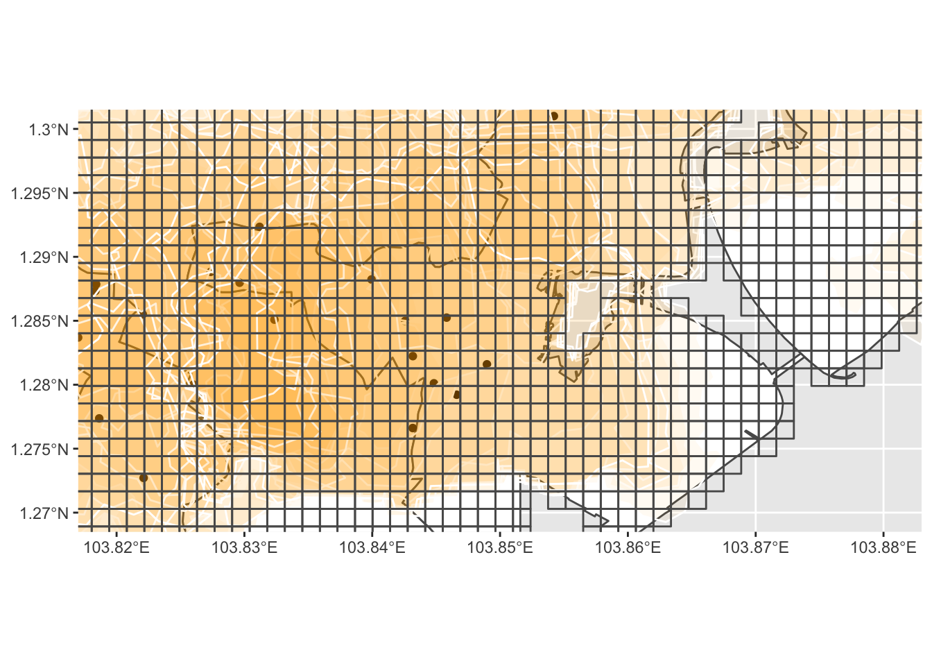
Next we overlay the geohash grid and the 114 different hawker isochrones to find out which isochrones intersect which geohashes. We then aggregate on the geohash level to count how many isochrones intersect, and the total number of stalls associated with each isochrone.
# Intersect geohashes and isochrones and tabulate intersecting details
hawker30_grid <- grid7 %>%
  st_join(hawker30, left = FALSE) %>%
  group_by(ID) %>%
  summarise(no_food_centres = n(),
            no_food_stalls = sum(no_food_stalls))
The downside is that this creates a large number polygons (~35k), which might cause some performance issues down the line. And as we can see, many of these polygons contain no useful information. One way we can work around this is to take advantage of geohashes inherent nesting structure and aggregate up the empty ones into larger geohashes where appropriate. This is done using a series of sf::st_covered_by across multiple grid layers, but in principle could also be done using just the characteristics of the string hashes that encode each geohash.
empty_grid6 <- grid6[lengths(grid6 %>%
  st_intersects(hawker30_grid, sparse = TRUE)) == 0,]

empty_grid7 <- grid7[lengths(grid7 %>% st_covered_by(empty_grid6, sparse = TRUE)) == 0,]

empty_grid7 <- empty_grid7[lengths(empty_grid7 %>% st_covered_by(hawker30_grid, sparse = TRUE)) == 0,]

# Visualize what this looks like
ggplot() +
  geom_sf(data = sg_map, fill = "black", colour = "black") +
  geom_sf(data = empty_grid6, fill = "white", colour = "grey20") +
  geom_sf(data = empty_grid7, fill = "orange", colour = NA) +
  geom_sf(data = hawker30_grid, fill = "navy", colour = NA)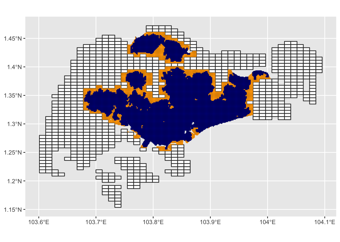
1-(length(empty_grid7$ID) +
  length(empty_grid6$ID) +
  length(hawker30_grid$ID))/length(grid7$ID)
## [1] 0.4787875We can see that this process reduced the number of polygons by almost half. The next step involves taking the geohashes with isochrone intersections and combining them back with the remaining geohashes that did not have any intersections that we just created above.
# Combine the intersecting geohashes and the non-intersecting ones together
hawker30_grid <- do.call(rbind,list(empty_grid7 %>%
  mutate(no_food_centres = 0, no_food_stalls = 0),
  empty_grid6 %>%
  mutate(no_food_centres = 0, no_food_stalls = 0),
  hawker30_grid))

# Visualize grids described by number of accessible food stalls
ggplot() +
  geom_sf(data = sg_map, fill = "white") +
  geom_sf(data = hawker30_grid, colour = "white", aes(fill = no_food_stalls), alpha = 0.75) +
  scale_fill_viridis_c() +
  xlim(c(103.82,103.88)) + ylim(c(1.27,1.3))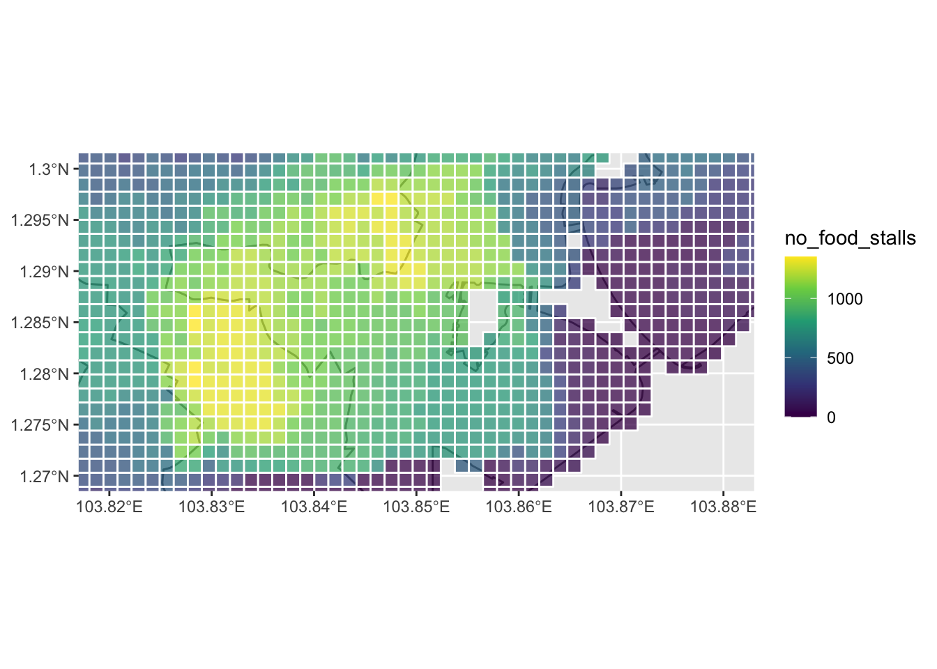
Making things interactive with mapdeck
Mapdeck is my one of my favourite R packages for making interactive web visualizations. Created by David Cooley, it uses Uber’s open-source deck.gl WebGL Javascript library for rendering spatial data alongside Mapbox’s tiling service.
As mapdeck uses tiles from Mapbox, it also requires a Mapbox API key, but you can use the same one specified for mapboxapi.
Mapdeck lets you create tooltips from HTML content, so we can supply some details viewable on mouseover by pasting together data alongside some basic HTML tags.
# Add HTML for interactive tooltips in mapdeck
hawker30_grid <- hawker30_grid %>%
  mutate(tooltip = paste0('Hawker stalls within a 30 min walk: <br>',no_food_stalls,
                          '<br>Hawker centers within a 30 min walk: <br>',
                          no_food_centres))

hawkers <- hawkers %>%
  mutate(
    original_completion_date = str_extract(Description,"(?<=<th>EST_ORIGINAL_COMPLETION_DATE</th> <td>)(.*?)(?=</td>)"),
    detail = str_extract(Description,"(?<=<th>DESCRIPTION_MYENV</th> <td>)(.*?)(?=</td>)"),
    clean_desc = paste0(
    name,'<br>Original completion date: <br>',original_completion_date,
    '<br>No. food stalls: <br>',no_food_stalls,
    '<br>No. market stalls: <br>',no_market_stalls,
    '<br>Description: <br>',detail))
Finally, the code below will produce the map at the top of the page, using the custom tooltips generated above.
library(mapdeck)
# Render in mapdeck
md <- mapdeck(
  style = mapdeck_style("dark"),
  zoom = 11.5,
  location =  c(103.8228077, 1.3014751)
) %>%
  add_polygon(
    data = hawker30_grid,
    layer = "polygon_layer",
    fill_colour = "no_food_stalls",
    fill_opacity = 0.75,
    tooltip = "tooltip",
    auto_highlight = FALSE,
    update_view = FALSE
  ) %>%
  add_scatterplot(
    data = hawkers,
    radius = 50,
    fill_colour = "#f57b42",
    layer_id = "scatter_layer",
    tooltip = "clean_desc",
    update_view = FALSE
  )

# Then wrap output in widgetframe::frameWidget() - https://github.com/SymbolixAU/mapdeck/issues/257
widgetframe::frameWidget(md)
And there you have it. Deck is great for fast and responsive web visualizations with a large number of geographic features, and the mapdeck package makes it very easy to work with. As always, this post is entirely on github and should be fully reproducible. If you have any questions, please contact me. If you have hawker stall recommendations, please comment. And if you found this interesting, please share on social media.